This article is part of the Security Tech Blog Series: Spring Cleaning for Security, brought to you by Simon from the Security Engineering team. We hope this article can provide you with some useful pointers to kickstart your journey in log anomaly detection, and get familiar with some of the techniques used at Mercari to identify log events of interest.
Warning: this article may contain traces of maths
Techniques used:
- Basic probability and mathematics (log2, z score)
- Information theory
- The Computerphile Youtube Channel published a nice introduction video on the subject
Infrastructure and languages used:
- Google Cloud Platform BigQuery (SQL)
- Python3, pandas dataframes, gcloud python libraries
Introduction
As a security professional, I can’t recall how many times I have been asked to detect anomalies in system logs. Expectations are often that we are able to read the mind of actors and detect their intent. After more than 20 years in the domain, telepathy is sadly a skill I’ve yet to acquire. Fortunately, there is some hope for achieving similar goals without having to delve into the supernatural or develop psychic powers.
The goal of this article is to introduce a method based on Information Theory that the Security team has been using at Mercari to detect less expected behaviors among users of a system, while building up the detection capabilities of our SOAR system. 1
TL;DR.
Extracting a list of top talkers (most active actors) from a set of logs is equivalent to giving each event a weight of "1" and sorting the actors by the number of actions they performed.
The weight assigned to each event doesn’t have to be "1". We can calculate an alternative weight by using -log2(p(x)) (the negative binary logarithm of probability of x) where p(x) is the probability of an event to be observed. Negative logarithmic functions have an inverting effect: small probabilities will render bigger values, while higher probabilities produce smaller values. This can be interpreted as the information value produced by each event. Summing up all these information values per actor can be a useful metric that gives an indication about the amount of information produced by each actor. The greater the sum, the more interesting the behavior should be.
Common Strategies
First, let’s define what we mean by an anomaly:
Anomaly
/əˈnɒm(ə)li/
- Something different, abnormal, peculiar, or not easily classified : something anomalous They regarded the test results as an anomaly.
- Deviation from the common rule : irregularity
- The angular distance of a planet from its perihelion as seen from the sun
Definition from the Merriam-Webster Dictionary
This means we are looking for something different, abnormal, peculiar, or not easily classified from a set of in random logs. But how would we normally go about this?
The method "à la mode du jour" would likely be machine learning. AWS uses the Random Cut Forest (RFC) Algorithm to analyze system activities as part of their GuardDuty service. This approach is definitely worth trying!
… but using something like this would involve having some servers with a trained model, building a data pipeline, etc., and I don’t want to take all this time to get everything setup. Is there not something that can be done just using SQL?
One common approach is to look for top talkers. Usual suspects will show up at the top, less interesting users will remain at the bottom of the list. Such an approach makes it easy and ideal to find someone suddenly crawling one of your systems.
Another method would be to calculate the average amount of events per a specified time window and trigger an alert if this amount goes over a certain threshold.
A more advanced method would be to ask a subject matter expert to assign a weight for each possible action, and then have the monitoring system calculate the sum of weighted actions for each user based on all their actions. This approach is often taken by anti-malware software. It implies that we have a clear idea of what is normal and what is not. The result is often highly specialized to detect specific types of events.
A Different Approach: Not All Data Has The Same Information Value
After looking at tons of event logs, it is obvious that not all events have the same value. Some events will provide more information value than others, and others will simply be discarded as mostly being noise.
We could identify and highlight the events that convey useful information and tone down the less useful ones. That’s normally what analysts will do over time as they become knowledgeable about a system.
Conveniently there is a shortcut, we can use a logarithm function (specifically log2) to calculate how many bits are required to represent certain information given the potential outcomes.
For example, if I flip a coin, there are two possible outcomes (ignoring the edge case where the coin can land on the… edge): Heads or Tails. This information can be represented by a single bit (0 or 1). If we were to store this in memory, we would need 1 bit (0 or 1). This can be evaluated by calculating the -log2 of probability 1/2.
import math

-math.log2(1/2)1.0Similarly, we can calculate how many bits would be needed to represent other probabilities.
print('Information value of...')
print('* 1d6 die landing on a 6: {:0.2f} bits'.format(-math.log2(1/6)))
print('* Winning at a 6/49 lottery: {:0.2f} bits'.format(-math.log2(1/14000000)))
print('\n* The letter E being used in the English Language: {:0.2f} bits'.format(-math.log2(13/100)))
print('* The letter Q being used in the English Language: {:0.2f} bits'.format(-math.log2(0.00095)))
print('\n* The Montreal Canadiens winning a game in 2021~2022: {:0.2f} bits'.format(-math.log2(24/56)))
print('* The Toronto Maple Leafs winning a game in 2021~2022: {:0.2f} bits'.format(-math.log2(35/56)))
print("  ^ Lately, it's less surprising to see Toronto winning more than Montreal :facepalm:")
print('\n* The Beastie Boys mentioning Macaroni and Cheese in one of their songs: {:0.2f} bits'.format(-math.log2(10/142)))
Information value of...
* 1d6 die landing on a 6: 2.58 bits
* Winning at a 6/49 lottery: 23.74 bits
* The letter E being used in the English Language: 2.94 bits
* The letter Q being used in the English Language: 10.04 bits
* The Montreal Canadiens winning a game in 2021~2022: 1.22 bits
* The Toronto Maple Leafs winning a game in 2021~2022: 0.68 bits
^ Lately, it's less surprising to see Toronto wins than Montreal :facepalm:
* The Beastie Boys mentioning Macaroni and Cheese in one of their songs: 3.83 bitsWhere are these bits coming from?
Here is the definition of information value from Wikipedia
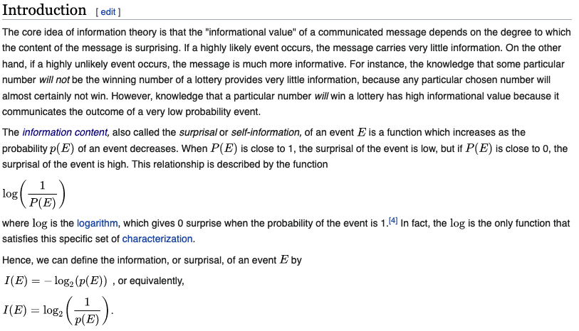
I will mostly be using the last equation to calculate the amount of information produced by events.
As we can see in the next cell, using logarithmic functions has an additional benefit: log of probabilities adds up, while probabilities have to be multiplied, which causes a problem. More on this later.
-math.log2(1/6) + -math.log2(1/6) + -math.log2(1/6) == math.log2(1/(1/6) * 1/(1/6) * 1/(1/6))TrueWhy would this be useful? If we think of the sum of all -log2 of probabilities as the amount of bits of information value representing all the actions of a user where more information is needed to represent less likely events, we can use this to sort by (un)likelihood that a user would take these actions.
Let’s see how this can be used with a simple scenario.
Scenario 1: Evaluating User Behavior
Context
We have a really simple ecommerce site where customers can login, search, buy items, and then get them delivered to their house.
We are asked to find out if the site is being attacked by malicious actors.
It’s your second day on the job, you don’t know the application, or what an attack would look like.
To build up this scenario, I will be using the pandas, numpy and math libraries from Python. matplotlib will be used to visualize some results.
For this example, we only have 8 users for which I am simulating a sequence of actions:
- 4 normal users
- 1 power users
- 3 malicious users
# some libraries are necessary for this next section
import pandas as pd
import numpy as np
import matplotlib.pyplot as plt
users = {
"user_1_normal": ['login:success'] + 5 * ['search'] + ['add payment method:success', 'buy:success'] + 3 * ['search'],
"user_2_normal": ['create account', 'add payment method:success', 'change delivery address'] + 4 * ['search'] + ['buy:success'] + 2 * ['search'] + ['buy:success'],
"user_3_normal": ['login:success'] + 12 * ['search'],
"user_4_normal": 2 * ['login:fail'] + ['login:success'] + 12 * ['search'] + ['buy:success'] + 4 * ['search'],
"user_5_power": ['login:success'] + 21 * ['search'] + ['buy:success'] + 2 * ['search'] + ['buy:success'] + 4 * ['search'] + ['buy:success'] + 9 * ['search'] + ['buy:success'],
"user_x_malicious": 3 * ['login:fail'] + ['login:success', 'change delivery address', 'search', 'buy:success', 'search', 'buy:success', 'search', 'buy:success', 'search', 'buy:fail'],
"user_y_malicious": 1 * ['login:fail'] + ['login:success'] + 2 * ['add payment method:fail'] + ['add payment method:success'] + 4 * ['add payment method:fail'] + ['add payment method:success'] + 1 * ['add payment method:fail'] + ['add payment method:success'],
"user_z_malicious": 12 * ['login:fail'] + ['login:success'],
}
all_activities = []
for u in users.keys():
all_activities = all_activities + users[u]
unique_actions = sorted(list(set(all_activities)))Sorting Users by Top Talkers
First, let’s look at the top talkers. The reasoning is that if someone is doing brute force on the login function, crawling the application, or spamming, they are likely to try to achieve that objective as fast as possible, creating a distinctive spike in our system’s logs.
The following loop will compile the activities of all users in a table format, ordered by the number of actions, as a search for top talkers would outline.
# Transform the user dictionary and sub-lists into a two dimension table where row = user and column = action.
actions_per_user = []
for u in users.keys():
    row = {x: users[u].count(x) for x in unique_actions}
    row['user'] = u
    row['total'] = len(users[u])
    actions_per_user.append(row)

# Pandas generates prettier tables than printing a dict. I use this opportunity to sort the rows by
# total number of actions
df_top = pd.DataFrame(actions_per_user).reindex(columns= ['user', 'total'] + unique_actions)\
    .sort_values(by='total', ascending=False) \
    .reset_index(drop=True)

# then we print the table
df_top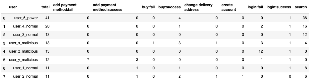
We can already see that the "search" action is widely used by most of the users.
Experts on the application could decide to filter out any "search" action and then maybe only focus on failures, but at this stage we don’t know yet if it’s important or not, so I will leave everything there.
In this case at least, simply sorting by the count of actions isn’t helping us identify the malicious activities quickly. If we were to take that list and go down from the top, it would take us some time to reach the first malicious user.
In this case, user_5 is a power user, and is generating a lot more noise than others. In a bigger application, we are likely to have a lot more of these users. The malicious users are actually showing up in the middle of the list, between normal users.
We can already have the instinct that not all actions have the same information value. This is where calculating the probability of each action, transforming this in bits through the log2 function, then calculating the sum of information value per user becomes useful.
Calculating the Sum of Information Value Produced By Each User
Somes basics about probabilities:
- Probabilities are represented by numbers between 0 and 1, where 0 means "zero chance", and 1 means "100%".
- When dealing with multiple probabilities, they multiply each other (if we naively assume that they are independent).
- For example: the probability of rolling a 6 three times on a 6 sided die can be calculated by multiplying 1/6 1/6 1/6 = 0.00462962962963, roughly ~0.46%.
To evaluate the probability of observing all the actions taken by a user, the first step is to find the probability of observing each action. The next cell will calculate these probabilities:
absolute_table = {x: all_activities.count(x) for x in unique_actions}
absolute_table = {k: v for k, v in sorted(absolute_table.items(), key=lambda absolute_table: absolute_table[1], reverse=True)}

probability_table = {x: all_activities.count(x)/len(all_activities) for x in unique_actions}

print("Absolute count and probability for each action (x/{} * 100)".format(len(all_activities)))
for action in absolute_table.keys():
    print("* {} ({:0.2f})%: {}".format(absolute_table[action], probability_table[action]*100, action))
Absolute count and probability for each actions (x/134 * 100)
* 82 (61.19)%: search
* 18 (13.43)%: login:fail
* 11 (8.21)%: buy:success
* 7 (5.22)%: add payment method:fail
* 7 (5.22)%: login:success
* 5 (3.73)%: add payment method:success
* 2 (1.49)%: change delivery address
* 1 (0.75)%: buy:fail
* 1 (0.75)%: create accountWith these probabilities calculated, we can go through each user and multiply all the probabilities for the actions they did. The result is the product of probabilities of all the actions observed. The smaller the product of probabilities the less likely that a user would perform these actions.
scored_users_prob = {u:1 for u in users.keys()}
for u in users:
    for a in users[u]:
        scored_users_prob[u] = scored_users_prob[u] * probability_table[a]

scored_users_prob = {k: v for k, v in sorted(scored_users_prob.items(), key=lambda scored_users_prob: scored_users_prob[1])}

print("Probability of observing all actions for a given user, based on the probability lookup table:")
for user in scored_users_prob.keys():
    print("#{}, {}, probability product: {:0.12f}%, number of actions: {}".format(
        list(scored_users_prob.keys()).index(user) + 1,
        user,
        scored_users_prob[user] * 100,
        len(users[user])
    ))
Probability of observing all actions for a given user, based on the probability lookup table:
#1, user_y_malicious, probability product: 0.000000000000%, number of actions: 12
#2, user_5_power, probability product: 0.000000000005%, number of actions: 41
#3, user_x_malicious, probability product: 0.000000000109%, number of actions: 13
#4, user_z_malicious, probability product: 0.000000000180%, number of actions: 13
#5, user_2_normal, probability product: 0.000000147067%, number of actions: 11
#6, user_4_normal, probability product: 0.000002991999%, number of actions: 20
#7, user_1_normal, probability product: 0.000314643502%, number of actions: 11
#8, user_3_normal, probability product: 0.014404622786%, number of actions: 13The malicious users are showing up at the top! It works! It’s magic! ^_^
… but we can see that we will end up with a problem if we use this method on bigger applications with greater number of actions. The number 1 in our list has a probability of 0.many0% with only 12 actions. Our float variables will likely round to 0, eventually breaking our sorting.
This is why it’s important to convert these probabilities into bits of information, using log2.
# Generating the lookup table with the information value in bits of each action
value_table = {x: -math.log2(all_activities.count(x)/len(all_activities)) for x in unique_actions}
value_table = {k: v for k, v in sorted(value_table.items(), key=lambda value_table: value_table[1], reverse=True)}

for action in value_table.keys():
    print("* {:0.3f}bits: {}".format(value_table[action], action))
* 7.066bits: buy:fail
* 7.066bits: create account
* 6.066bits: change delivery address
* 4.744bits: add payment method:success
* 4.259bits: add payment method:fail
* 4.259bits: login:success
* 3.607bits: buy:success
* 2.896bits: login:fail
* 0.709bits: searchWe can interpret these bits as the information value — i.e an indicator of how much we should be surprised to see any given action. In this case, the "search" action being observed doesn’t even worth 1 bit of information. If someone is hammering the "search" function over and over, this is still something we would want to know about. Not giving a score of 0 then makes sense.
We now have a way to automatically calculate a naive scoring table for each action. The values will always be greater than 0. More common (noisy) actions will still count, but will score lower than the less likely ones.
Side note about continuous values:
This method only works on a discrete set of events. It would likely fail on numbers (integers or floats) since using continuous numbers would render a lookup table where each value would have a 1/n probability of happening. A potential hack is to append a number to the action performed by each user, the equation
10^(ceil(log10(x)))rounds the number to the lowest power of 10. In this example, we would see something likebuy:10:success,buy:1000:success,buy:10000:fail.
Let’s apply this to our previous scenario.
For each of the actions performed by our users, we sum all the information value for their actions. The higher the sum, the less likely we are to see a user doing these actions, thus the more abnormal we can consider the user’s behavior to be.
scored_users_bits = {u:0 for u in users.keys()}

for u in users:
    scored_users_bits[u] = sum(
        [value_table[action] if action in value_table.keys() else -math.log2(1/len(all_activities))
         for action in users[u]]
    )

scored_users_bits = {k: v for k, v in sorted(scored_users_bits.items(), key=lambda scored_users_bits: scored_users_bits[1], reverse=True)}

for user in scored_users_bits.keys():
    print("#{}, user: {}, entropy: {:0.1f}bits, number of actions: {}".format(
        list(scored_users_bits.keys()).index(user)+1,
        user,
        scored_users_bits[user],
        len(users[user])
    ))
#1, user: user_y_malicious, entropy: 51.2bits, number of actions: 12
#2, user: user_5_power, entropy: 44.2bits, number of actions: 41
#3, user: user_x_malicious, entropy: 39.7bits, number of actions: 13
#4, user: user_z_malicious, entropy: 39.0bits, number of actions: 13
#5, user: user_2_normal, entropy: 29.3bits, number of actions: 11
#6, user: user_4_normal, entropy: 25.0bits, number of actions: 20
#7, user: user_1_normal, entropy: 18.3bits, number of actions: 11
#8, user: user_3_normal, entropy: 12.8bits, number of actions: 13The resulting list has the same order as the one produced using the product of probabilities, without the floating point overflow problem.
The following table shows the sum of bits of information per user. Earlier with the Top Talker method, the "search" action had the greatest count. Here, we still grant some value for "search" actions, but they are significantly less than the "add payment method:fail" or "login:fail" actions.
Just presenting the sum of bits might make it hard to know what can really be considered as high or not. For this, I will calculate the z score for each.
Side note: What is this a z score?
The zscore is the number of standard deviations of a value against the mean of the values being measured.
zscore = (cnt – mean) / std
- where cnt is the count of events for an actor (here: users)
- mean is the average number of cnt for all the actors
- std is the standard deviation of cnt for all the actors
actions_per_user = []
for u in users.keys():
    row = {action: users[u].count(action) * value_table[action] for action in unique_actions}
    row['user'] = u
    row['bits'] = sum([value_table[action] for action in users[u]])
    row['cnt'] = len(users[u])
    actions_per_user.append(row)

df = pd.DataFrame(actions_per_user)
mean = df['bits'].mean()
std = df['bits'].std()
df['zscore'] = (df['bits'] - mean)/std
print('mean: {:0.2f}, std: {:0.2f}'.format(mean, std))mean: 32.44, std: 13.31df = df.reindex(columns= ['user', 'cnt', 'bits', 'zscore'] + unique_actions).round(decimals=2)
df.sort_values(by='zscore', ascending=False)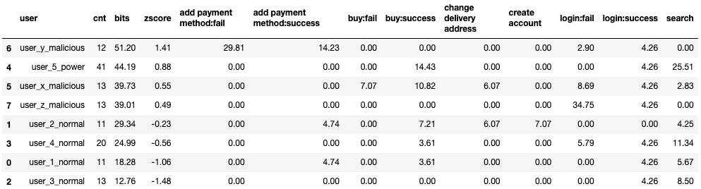
def graph_distribution(df, x_axis, y_axis, labels):
    fig, ax = plt.subplots(figsize=(15,4))
    x = df[x_axis].values
    y = df[y_axis].values
    l = df[labels].values

    ax.scatter(x, y)
    for i, txt in enumerate(l):
        ax.annotate(txt, (x[i], y[i]))
    plt.xlabel('zscore')
    plt.ylabel('count of events')
    plt.title('Scatter plot of zscore by count of events')

    return plt

plt = graph_distribution(df, 'zscore', 'cnt', 'user')
plt.show()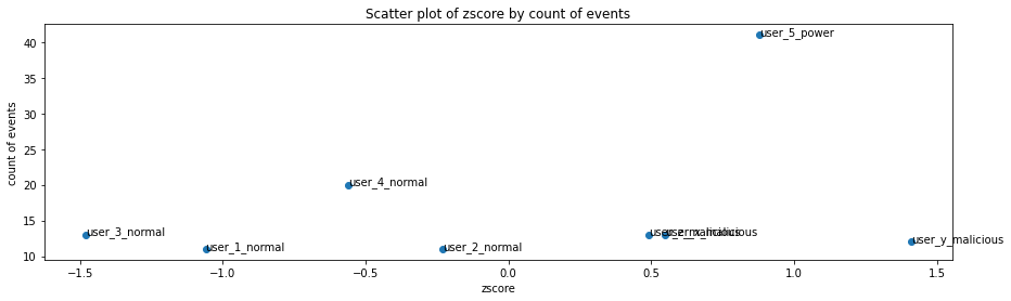
Here I use the zscore to demonstrate how far away each user is from the average.
- A zscore of 0 means that the user has a count of events equal to the average. 50% of the users are less noisy.
- A zscore greater than 1 means that these users are in the top 15.8%. 84.1% of the users are less noisy.
- A zscore greater than 2 means that these users are in the top 2.3%. 97.7% of the users are less noisy.
- A zscore greater than 3 means that these users are in the top 0.1%. 99.9% of the users are less noisy.
In this example, the difference of the information value between each user isn’t much, but we can already see that normal users will tend to have negative z scores, while malicious and power users will have a z score greater than 0, with the top malicious user (user_y with 51.2 bits) is at 1.41 standard deviations from the mean (32.44).
This z score will come in handy when we have a large quantity of users and a wider spread of values. Using it isn’t necessary, just a convenient way to set thresholds.
If we compare both the top talker and bits sorting methods, we can clearly see that the sorting changes significantly.
rows = []
for user in scored_users_bits.keys():
    rows.append({
        "user": user,
        "toptalker": list(df_top['user']).index(user),
        "bits": list(scored_users_bits.keys()).index(user),
        "delta": list(df_top['user']).index(user) - list(scored_users_bits.keys()).index(user)
    })
pd.DataFrame(rows) 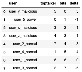
In the next section, I will demonstrate how to use this method with data stored in BigQuery using SQL queries, making it (relatively) easy to adapt to any kind of discrete data. The surrounding Python code is mainly used to demonstrate my point, and is an optional read.
Some Important Details to Keep in Mind
This approach provides an alternative scoring method to the normal "1 action, 1 point" scoring method that the Top Talker technique uses implicitly.
When the importance of each action isn’t always known, naively assigning an information value based on the probability of seeing each action to be observed can be a good starting point. Actors (users, IP addresses, etc.) producing more information value than the others will then show up at the top of our list.
This method helps in identifying what might be more interesting to look at first. The top of the list will not necessarily be malicious activities. Through an iterative process, actions and users that are identified as normal (not interesting) can be filtered out before running the analysis again. The result will likely be more interesting over time as only useful actions are used to calculate the information values.
In the previous example, and in the following example, I am using the same data to calibrate the information value of each event. To detect anomalies in logs, training on a different time window is likely to produce better results.
Scenario 2: Shakespeare’s Corpus
The first scenario demonstrated how to calculate the information value from user actions. This method can also be applied to other use cases. In this section, I will be using the number of occurrences of each word from Shakespeare’s corpus, available as a public dataset on BigQuery. The result isn’t really useful, but a fun way to compare the information value of each piece of work, based on the probability of each words being used.
This method could also be used to compare lyrics of different artists for example. The difference of information gained can be evaluated by using Kullback-Leibler divergence, but I will leave this as a homework exercise for any readers keen to try out that technique.
First, I need to import the necessary libraries to query BigQuery:
%load_ext autoreload
%autoreload 2

import warnings
warnings.filterwarnings("ignore")

try:
    from google.cloud import bigquery
    from anon_functions import gcp_project
    client = bigquery.Client(project=gcp_project)
except:
    print("disconnected mode")

from anon_functions import compare_models
The following query will be used to retrieve the data from BigQuery:
shakespear_sql = """
    SELECT
      corpus, LOWER(word) AS word, SUM(word_count) AS cnt
    FROM
      `bigquery-public-data.samples.shakespeare`
    GROUP BY
      corpus, LOWER(word)
"""

df_shakespeare = client.query(shakespear_sql).to_dataframe()
To compare the frequencies of each word, I am adding the z score in the next cell.
def add_zscore_to_df(df):
    df_per_user = df.groupby(['corpus']).agg({'cnt': ['sum']})
    mean = df_per_user['cnt'].mean()
    std = df_per_user['cnt'].std()
    df_per_user['zscore'] = (df_per_user['cnt'] - mean)/std

    print('mean: {}, std: {}'.format(mean.values, std.values))
    return df_per_user.sort_values(by=('cnt', 'sum'), ascending=False).reset_index()

df_shakespeare_per_corpus = add_zscore_to_df(df_shakespeare)

pd.options.display.max_rows = 20
df_shakespeare_per_corpus
mean: [22520.11904762], std: [6411.87254032]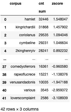
If we graph each corpus by their count of words against the z score, we can see that the result is a straight line, directly correlated to the number of words per corpus.
plt = graph_distribution(df_shakespeare_per_corpus, 'zscore', 'cnt', 'corpus')
plt.show()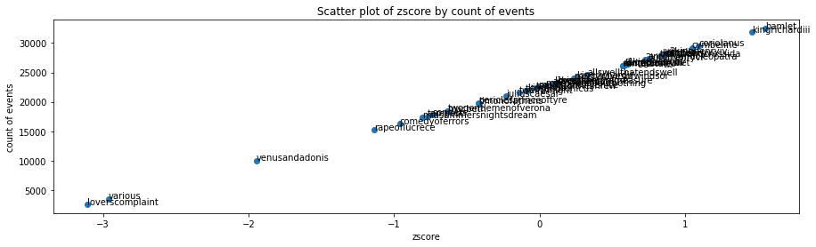
Which words are the most common? The next cell lists the top ones:
top_words = df_shakespeare.groupby(['word']).agg({'cnt': ['sum']}).reset_index().sort_values(by=('cnt', 'sum'), ascending=False).head(10)['word'].values
top_corpus = df_shakespeare.groupby(['corpus']).agg({'cnt': ['sum']}).reset_index().sort_values(by=('cnt', 'sum'), ascending=False).head(10)['corpus'].values

df_shakespeare[(df_shakespeare['word'].isin(top_words)) & df_shakespeare['corpus'].isin(top_corpus)].pivot_table(
    index=['corpus'],
    columns='word',
    values='cnt',
    aggfunc=np.sum,
    fill_value=0
)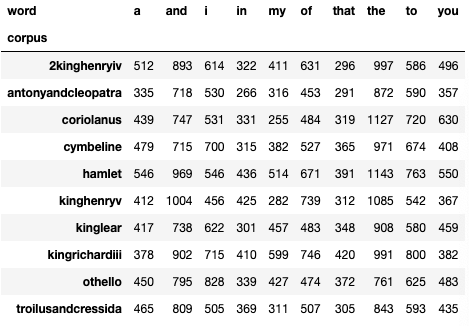
These aren’t the most interesting words…
Let’s calculate the information value for each of the words present in the documents
unique_words = list(df_shakespeare['word'].unique())
all_words = sorted(list(df_shakespeare['word'].values))
counted_words = {x: all_words.count(x) for x in unique_words}

value_table = {x: -math.log2(counted_words[x]/len(all_words)) for x in unique_words}
value_table = {k: v for k, v in sorted(value_table.items(), key=lambda value_table: value_table[1], reverse=True)}

for word in list(value_table.keys())[:5]:
    print("* {:0.3f}bits: {}".format(value_table[word], word))

print('... ', len(value_table.keys()) - 20, 'more ...')

for word in list(value_table.keys())[-5:]:
    print("* {:0.3f}bits: {}".format(value_table[word], word))
* 17.168bits: lvii
* 17.168bits: w
* 17.168bits: happies
* 17.168bits: enjoyer
* 17.168bits: disarm'd
... 26908 more ...
* 11.775bits: heart
* 11.775bits: eyes
* 11.775bits: for
* 11.775bits: but
* 11.775bits: iCreating this lookup table can be done automatically within the SQL query, then be used to calculate the sum of information value for each corpus.
- "words": The first part is the query we used earlier.
- "all_words": the second part is needed to calculate the total amount of words present in all corpus. It is needed to calculate the probability of each word.
- "lookup_table": The third part will calculate the information value of each word
- … and the last query sums up all the values
shakespear_bits_sql = """
WITH
  words AS (
    SELECT
      corpus, LOWER(word) AS word, SUM(word_count) AS cnt
    FROM
      `bigquery-public-data.samples.shakespeare`
    GROUP BY
      corpus, LOWER(word)
  ),
  all_words AS (
    SELECT
      SUM(cnt) AS cnt
    FROM
      words
  ),
  lookup_table AS (
    SELECT
      b.cnt AS total,
      a.word AS word,
      -LOG(SUM(a.cnt)/b.cnt,2) AS bits
    FROM
      words a
    JOIN all_words b ON 1=1
    GROUP BY
      a.word, b.cnt
  )
SELECT
  words.corpus, SUM(words.cnt) AS cnt, SUM(lookup_table.bits) AS bits
FROM
  words
JOIN lookup_table ON words.word = lookup_table.word
GROUP BY
  corpus
ORDER BY bits DESC
"""

df_shakespeare_scored = client.query(shakespear_bits_sql).to_dataframe()
mean = df_shakespeare_scored['bits'].mean()
std = df_shakespeare_scored['bits'].std()
df_shakespeare_scored['zscore'] = (df_shakespeare_scored['bits'] - mean)/std
df_shakespeare_scored = df_shakespeare_scored.sort_values(by='zscore', ascending=False).reset_index(drop=True)
df_shakespeare_scored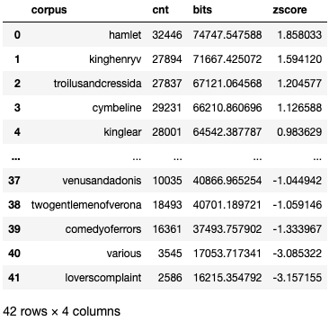
plt = graph_distribution(df_shakespeare_scored, 'zscore', 'cnt', 'corpus')
plt.show()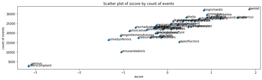
# Comparing the ranking of each corpus against the top talker method and information value method
compare_models(df_shakespeare_per_corpus, df_shakespeare_scored, df_shakespeare_per_corpus['corpus'], 'corpus').head(20)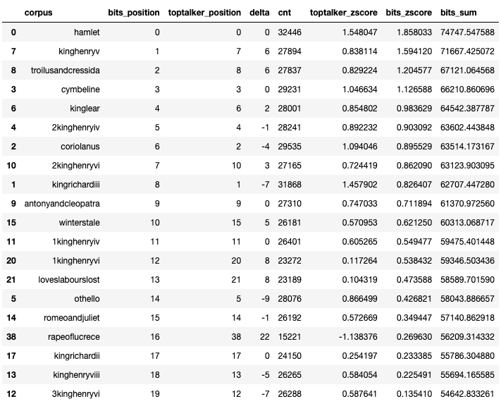
In conclusion, we can see that Hamlet is a masterpiece regardless if we are looking at it through simple word count or information value content, while some others are getting declassified.
This is obviously a silly example, but it proves that this technique could be used to weight the information content of tweets, messages, documents, and figure out which one contains something worth of attention.
In the next section, I will apply this technique on access logs from our Google Workspace API to demonstrate what we can learn from them.
Scenario 3: Google Workspace Logs
Calculating information value in the last two examples was fun, but how can this method be applied to a more real world scenario?
Context:
An insider decided to abuse the API of Google Workspace to search for documents containing potentially sensitive information. Can we find him?
This is a fictional context, but it is based on real activities. As part of our internal Chaos Security efforts, Maximilian worked on automating document content discovery. Let’s see if we can outline these actions.
Spoiler: It will (mostly) fail to bring Maximilian’s activities to the top of the list, because we will see that there are other activities that may be more worthy of attention.
First, I start by importing the necessary sanitization libraries to protect the identity of the innocents systems and users.
try:
    from anon_functions import gsuite_dataset, gsuite_noisy_apps
except:
    gsuite_noisy_apps = ["/*noisy_apps*/"]
    gsuite_dataset = '/*bigquery.gsuite_dataset*/'

try:
    from anon_functions import anonymize_email, anonymize_ip
except:
    def anonymize_email(email):
        return {"email": email}

    def anonymize_ip(ip):
        return ip

sanitized_gsuite_dataset = '/*bigquery.gsuite_dataset*/'
sanitized_noisy_apps = '"/*noisy apps*/"'
string_of_noisy_apps = '"' + '","'.join(gsuite_noisy_apps) + '"'

def sanitize_gsuite_query(sql):
    return sql.replace(gsuite_dataset, sanitized_gsuite_dataset).replace(string_of_noisy_apps, sanitized_noisy_apps)

def anon_gsuite_dataframe(df):
    df_anon = df.copy()
    if "actor" in df.columns:
        df_anon['actor'] = df_anon['actor'].apply(lambda x: anonymize_email(x)['email'])
    return df_anon

def add_zscore_to_df(df):
    df_per_user = df.groupby(['actor']).agg({'cnt': ['sum']})
    mean = df_per_user['cnt'].mean()
    std = df_per_user['cnt'].std()
    df_per_user['zscore'] = (df_per_user['cnt'] - mean)/std

    return df_per_user.sort_values(by=('cnt', 'sum'), ascending=False).reset_index()
Our activity occurred near the end of April.
investigation_start_date = "2022-04-24" # UTC, includes from 00:00:00
investigation_end_date = "2022-04-27" # UTC, includes until 23:59:59
The next cell contains the template of the query I will be using to extract actions from BigQuery. I am using a concatenation of multiple fields to create a distinct action field because actions need to be discrete, yet relevant. The resulting actor and action string can be interpreted as "Actor X does action Y on service Z", with a count of observations of that specific action.
I am also filtering out known noisy applications, which I recommend doing over multiple iterations. Once the result contains a relatively expected output, any significant deviation from it should be a good indicator that something is happening.
gsuite_event_sql = """
    SELECT
      email AS actor,
      CONCAT(
        event_name,
        ", ", token.app_name,
        ", ", token.api_name,
        ", ", token.method_name,
        ", ", token.product_bucket,
        ", ", token.client_type
      ) AS action,
      COUNT(time_usec) AS cnt
    FROM
      `{dataset}`
    WHERE
      DATE(_PARTITIONTIME) BETWEEN "{start}" AND "{end}"
      AND ip_address IS NOT NULL
      AND token.client_id IS NOT NULL
      AND token.api_name IS NOT NULL
      AND token.app_name NOT IN ({noise})
    GROUP BY actor, action
"""
I can now fill the template with the necessary parameters, then query BigQuery to recover the data.
gsuite_investigation_sql = gsuite_event_sql.format(
    dataset = gsuite_dataset,
    start = investigation_start_date,
    end = investigation_end_date,
    noise = string_of_noisy_apps
)
print(sanitize_gsuite_query(gsuite_investigation_sql))

df_gsuite_all = client.query(gsuite_investigation_sql).to_dataframe()
df_gsuite_all_anon = anon_gsuite_dataframe(df_gsuite_all)
SELECT
email AS actor,
CONCAT(
event_name,
", ", token.app_name,
", ", token.api_name,
", ", token.method_name,
", ", token.product_bucket,
", ", token.client_type
) AS action,
COUNT(time_usec) AS cnt
FROM
/*bigquery.gsuite_dataset*/
WHERE
DATE(_PARTITIONTIME) BETWEEN "2022-04-24" AND "2022-04-27"
AND ip_address IS NOT NULL
AND token.client_id IS NOT NULL
AND token.api_name IS NOT NULL
AND token.app_name NOT IN ("/*noisy apps*/")
GROUP BY actor, actiondf_gsuite_all_per_user = add_zscore_to_df(df_gsuite_all)
df_gsuite_all_per_user = df_gsuite_all_per_user.sort_values(by='zscore', ascending=False).reset_index(drop=True)
df_gsuite_all_per_user_anon = anon_gsuite_dataframe(df_gsuite_all_per_user.copy())
df_gsuite_per_user_top = df_gsuite_all_per_user_anon[df_gsuite_all_per_user_anon['zscore'] >= 2]
df_gsuite_per_user_top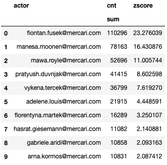
This last table contains the list of top talkers. The threshold of "number of actions" is set to 2 standard deviations over the mean. Anything under a zscore of 2 (bottom 97.7%) is considered as less relevant for now.
If we graph the frequency of all users with each count of actions, we can see that the number of actions per user is highly skewed to the left, explaining why the top one has such a high z score.
df_gsuite_all_per_user_anon[['actor', 'cnt']].plot.hist(grid=True)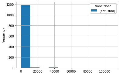
If we graph against the z score, we can see that most of the users are on the left.
plt = graph_distribution(df_gsuite_all_per_user_anon, 'zscore', 'cnt', 'actor')
plt.show()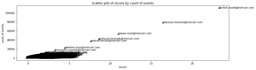
Where is our suspect in all this? We can find him at position 104.
df_gsuite_all_per_user_anon[df_gsuite_all_per_user_anon['actor'].isin(['suspect.szymkiewicz@mercari.com'])]| actor | cnt | zscore | |
|---|---|---|---|
| sum | |||
| 103 | suspect.szymkiewicz@mercari.com | 2529 | 0.31887 |
Let’s see what result we can find if we calculate the information value of each user.
Like for machine learning, it is preferable to train the model on a different dataset. I semi randomly selected 20 days prior to the investigation period, hoping that the probability distribution would be relatively stable.
training_start_date = "2022-04-01" # UTC, includes from 00:00:00
training_end_date = "2022-04-20" # UTC, includes until 23:59:59Here is the template I will be using to classify each user.
The blocks for the training_period and investigation_period use the same query presented earlier. For the rest, it is mostly the same query used for the Shakespeare example, with the exception that I will handle missing actions from the lookup table as unique actions, giving them a likelihood of 1/(total of all investigated actions). This is a naive assumption that there will be no more events of the same kind, but it has the advantage of highlighting the fact that the event was unexpected.
information_sql = """
WITH
training_period AS (
{training_sql}
),
training_everything AS (
SELECT SUM(cnt) AS cnt FROM training_period
),
lookup_table AS (
SELECT
a.action AS action,
LOG(1/(SUM(a.cnt) / b.cnt),2) AS bits
FROM
training_period a JOIN training_everything b ON 1=1
GROUP BY a.action, b.cnt
),
investigation_period AS (
{investigation_sql}
),
investigation_actor AS (
SELECT actor, SUM(cnt) AS cnt, FROM investigation_period GROUP BY actor
),
investigation_everything AS (
SELECT SUM(cnt) AS cnt FROM investigation_period
)
SELECT
investigation_period.actor,
SUM(investigation_period.cnt) AS cnt,
SUM(CASE
WHEN lookup_table.bits > 0
THEN lookup_table.bits
ELSE -LOG(1/investigation_everything.cnt,2)
END
) AS bits
FROM
investigation_period
LEFT JOIN lookup_table ON investigation_period.action = lookup_table.action
LEFT JOIN investigation_actor ON investigation_period.actor = investigation_actor.actor
JOIN investigation_everything ON 1=1
GROUP BY
investigation_period.actor
"""After parameterizing the templates, we can run the query.
gsuite_training_sql = gsuite_event_sql.format(
dataset=gsuite_dataset,
start=training_start_date,
end=training_end_date,
noise = string_of_noisy_apps
)
gsuite_query_sql = information_sql.format(
training_sql = gsuite_training_sql,
investigation_sql = gsuite_investigation_sql)
print(sanitize_gsuite_query(gsuite_query_sql))
df_gsuite_scored = client.query(gsuite_query_sql).to_dataframe()WITH
training_period AS (
SELECT
email AS actor,
CONCAT(
event_name,
", ", token.app_name,
", ", token.api_name,
", ", token.method_name,
", ", token.product_bucket,
", ", token.client_type
) AS action,
COUNT(time_usec) AS cnt
FROM
/*bigquery.gsuite_dataset*/
WHERE
DATE(_PARTITIONTIME) BETWEEN "2022-04-01" AND "2022-04-20"
AND ip_address IS NOT NULL
AND token.client_id IS NOT NULL
AND token.api_name IS NOT NULL
AND token.app_name NOT IN ("/*noisy apps*/")
GROUP BY actor, action
),
training_everything AS (
SELECT SUM(cnt) AS cnt FROM training_period
),
lookup_table AS (
SELECT
a.action AS action,
LOG(1/(SUM(a.cnt) / b.cnt),2) AS bits
FROM
training_period a JOIN training_everything b ON 1=1
GROUP BY a.action, b.cnt
),
investigation_period AS (
    SELECT
      email AS actor,
      CONCAT(
        event_name,
        ", ", token.app_name,
        ", ", token.api_name,
        ", ", token.method_name,
        ", ", token.product_bucket,
        ", ", token.client_type
      ) AS action,
      COUNT(time_usec) AS cnt
    FROM
      /*bigquery.gsuite_dataset*/
    WHERE
      DATE(_PARTITIONTIME) BETWEEN "2022-04-24" AND "2022-04-27"
      AND ip_address IS NOT NULL
      AND token.client_id IS NOT NULL
      AND token.api_name IS NOT NULL
      AND token.app_name NOT IN ("/*noisy apps*/")
    GROUP BY actor, action
),
investigation_actor AS (
SELECT actor, SUM(cnt) AS cnt, FROM investigation_period GROUP BY actor
),
investigation_everything AS (
SELECT SUM(cnt) AS cnt FROM investigation_period
)
SELECT
investigation_period.actor,
SUM(investigation_period.cnt) AS cnt,
SUM(CASE
WHEN lookup_table.bits > 0
THEN lookup_table.bits
ELSE -LOG(1/investigation_everything.cnt,2)
END
) AS bits
FROM
investigation_period
LEFT JOIN lookup_table ON investigation_period.action = lookup_table.action
LEFT JOIN investigation_actor ON investigation_period.actor = investigation_actor.actor
JOIN investigation_everything ON 1=1
GROUP BY
investigation_period.actormean = df_gsuite_scored['bits'].mean()
std = df_gsuite_scored['bits'].std()
df_gsuite_scored['zscore'] = (df_gsuite_scored['bits'] - mean)/std
df_gsuite_scored = df_gsuite_scored.sort_values(by='zscore', ascending=False).reset_index(drop=True)
df_gsuite_scored_anon = anon_gsuite_dataframe(df_gsuite_scored.copy())
df_gsuite_scored_top = df_gsuite_scored_anon[df_gsuite_scored_anon['zscore'] >= 2]
df_gsuite_scored_top.head(20)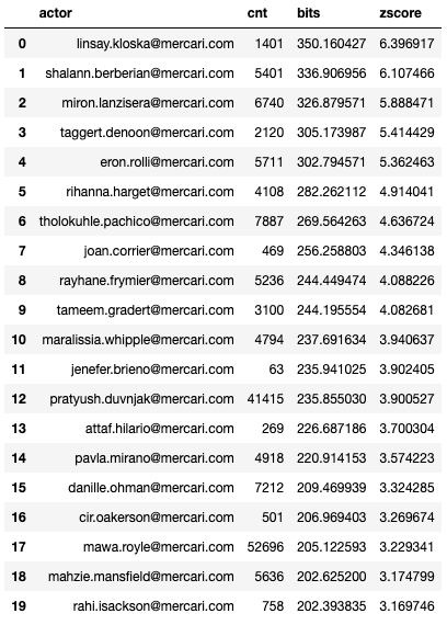
plt = graph_distribution(df_gsuite_scored_anon, 'zscore', 'cnt', 'actor')
plt.show()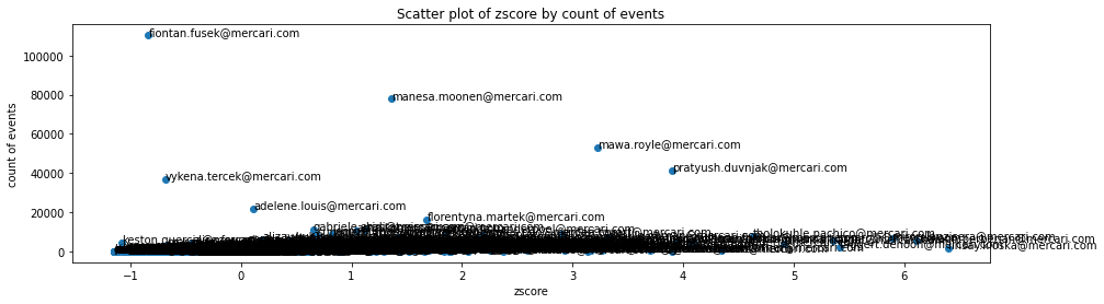
The actor ranking looks completely different from the top talker one. Graphing the count of events by the z score also shows a completely different picture. Top talkers still show up at the top of the graph, but on the left side, indicating less interesting activities, while users with a higher information value will show up on the lower right side.
Displaying the ranking of both models side by side shows how the ranking changed based on the information value.
df_compare = compare_models(df_gsuite_all_per_user_anon, df_gsuite_scored_anon, df_gsuite_scored_anon['actor'].unique())
df_compare.head(20)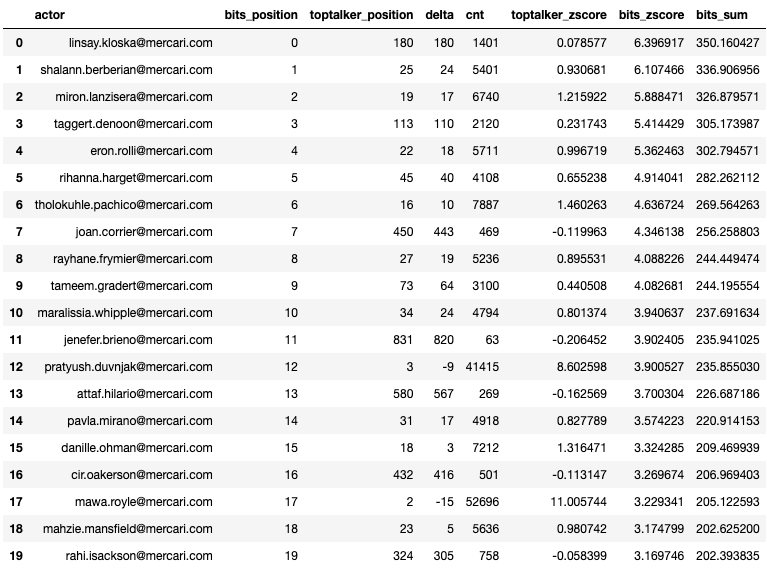
Investigating these users shows that many had connected OAuth applications to their account, mainly for calendar and drive functionality.
Why is this useful? By studying these users we can that we have multiple 3rd party applications connected to our systems. This is exposing some of the supply chain risks that we are facing and lacked visibility on before.
Meanwhile, where is our malicious user?
df_gsuite_scored_anon[df_gsuite_scored_anon['actor'] == 'suspect.szymkiewicz@mercari.com']| actor | cnt | bits | zscore | |
|---|---|---|---|---|
| 95 | suspect.szymkiewicz@mercari.com | 2529 | 121.412545 | 1.401142 |
Moving from position 104 to position 95 isn’t really impressive. Still it demonstrates that the activities done by our insider scored higher than when we were just looking at top talkers.
Conclusion
As we could see through these three scenarios, calculating the information value created by users produces a completely different, arguably more interesting output. However, this is still not magic. We naively assigned an information value to each action based on their probability of being observed. If we wanted to only score users against events that are relevant from a security point of view, we would need to filter out all other actions.
In any case, the produced output should highlight something potentially anomalous events/actions worth investigating. Through multiple iterations, queries can be tuned to filter out known irrelevant (from a security point of view) actions or actors, producing a more relevant classification over time.
If you found this blog interesting and want to work with us, we are hiring.
Further Reading / Watching
-
Blog Post by David Chapdelaine Detection Engineering and SOAR at Mercari
-
Blog Post by Maximilian Frank Terraform CI code execution restrictions
-
Introduction to Information Theory on Wikipedia
-
Why Information Theory is Important – Computerphile on Youtube
-
Kullback-Leibler divergence on Wikipedia